
Implementing Semantic Pareidolia via Direct Image Optimization
Gal Lahat

Abstract
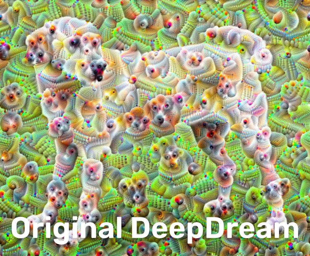
In 2015, Google released “DeepDream,” a computer vision program that popularized the concept of neural pareidolia, forcing a network to find patterns in an image and exaggerate them. While visually striking, DeepDream was fundamentally limited by its architecture: it was a discriminator trained to classify rigid objects like dogs and cars. It could only hallucinate what it had previously categorized.
This report explores the modern evolution of this technique. By replacing the classifier with a multimodal embedding model (CLIP), we can move from “finding dogs” to “finding concepts.” We introduce an architecture for Direct Latent Optimization that utilizes a Vision Transformer backbone, a “Cutout” view strategy, and a “Topology-Aware” regularization method. This approach allows us to mathematically coerce an image to embody abstract semantics, such as “love” or “space”, while strictly preserving the structural integrity of the original input, a task where modern diffusion models often struggle.
1. Introduction: Generation vs. Optimization
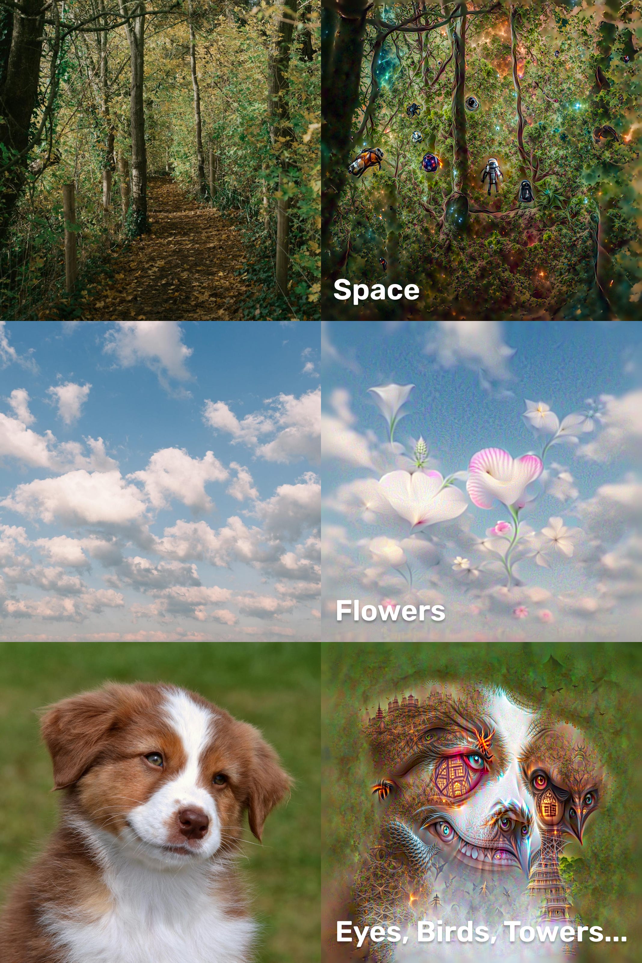
The current standard of AI art is dominated by Diffusion Models (like Stable Diffusion). These models work via reconstruction: they take pure noise and iteratively denoise it to match a text prompt. While powerful, it builds a new image from scratch. If you feed it a picture of a forest and ask for “space,” it will likely generate a generic nebula, discarding the specific layout of your original trees.
Direct Optimization works backwards. We do not generate new pixels. We take the existing pixels of an image and treat them as trainable variables. We then slide those pixels along a mathematical gradient until they satisfy a semantic condition. We are not painting a new picture; we exaggerate patterns in the existing data to make it look like something else.
2. The Engine: Contrastive Language-Image Pre-training (CLIP)
To understand how we steer the image, we must understand the compass: CLIP.
Standard classifiers (like ResNet trained on ImageNet) output a probability distribution across a fixed set of labels (e.g., “70% Beagle, 30% Muffin”). CLIP, however, is trained on 400 million image-text pairs using Contrastive Learning.
The model consists of two encoders:
The Image Encoder (I): Compresses an image into a vector.
The Text Encoder (T): Compresses text into a vector.
During training, CLIP is rewarded when the vector of an image aligns with the vector of its description. This forces the model to learn a shared 1024-dimensional latent space where the direction of the vector represents semantic meaning.
In our architecture, we freeze CLIP. We input our image (I) and our prompt (T). We then calculate the Cosine Similarity between their embeddings:
Our objective function is simple: maximize this similarity. We calculate the gradient of the similarity with respect to the pixels, effectively asking the model: “Which way should I push the RGB values of this pixel to make the image mathematically more ‘loving’?”
3. The Objective: Training the Pixels
This is where the magic happens. In a standard AI training loop, you show the model an image, check if it guessed right, and then update the Model’s Brain (Weights) to be smarter next time.
We do the exact opposite.
We freeze the model’s brain. We refuse to let it learn anything new. Instead, we update the Image (Pixels).
Here is the process, step-by-step:
Encode the Prompt: We feed our text (”Love, hearts, loving”) into CLIP. It outputs a coordinate in 1024-dimensional space. Let’s call this the Target Vector (T).
Encode the Image: We feed our starting image (the forest) into CLIP. It outputs a different coordinate. Let’s call this the Current Vector (I).
Calculate the Distance: We measure the angle between these two vectors using Cosine Similarity.
If the vectors point in the same direction, the Loss is 0. If they point in opposite directions, the Loss is high.
Backpropagate to Input: This is the key mathematical trick. We calculate the gradient of the Loss, but instead of applying it to the neural network layers, we travel all the way back to the RGB input tensor.
We ask the mathematical question: “How do I change this specific green pixel to make the total vector point 1% closer to ‘Love’?”
The optimizer (Adam) answers this question for every single pixel, thousands of times per second, slowly dragging the image through the latent space until the forest mathematically aligns with the concept of love.
4. Seeing the Big Picture: Vision Transformers
The original DeepDream relied on Convolutional Neural Networks (CNNs). CNNs process images using sliding windows (kernels). They are excellent at detecting textures (fur, eyes, scales) but struggle with global context. This is why DeepDream images often look like a mosaic of disconnected eyes.
Our implementation utilizes Large Vision Transformer. Unlike CNNs, Transformers utilize Self-Attention mechanisms. This allows every patch of the image to mathematically “attend” to every other patch.
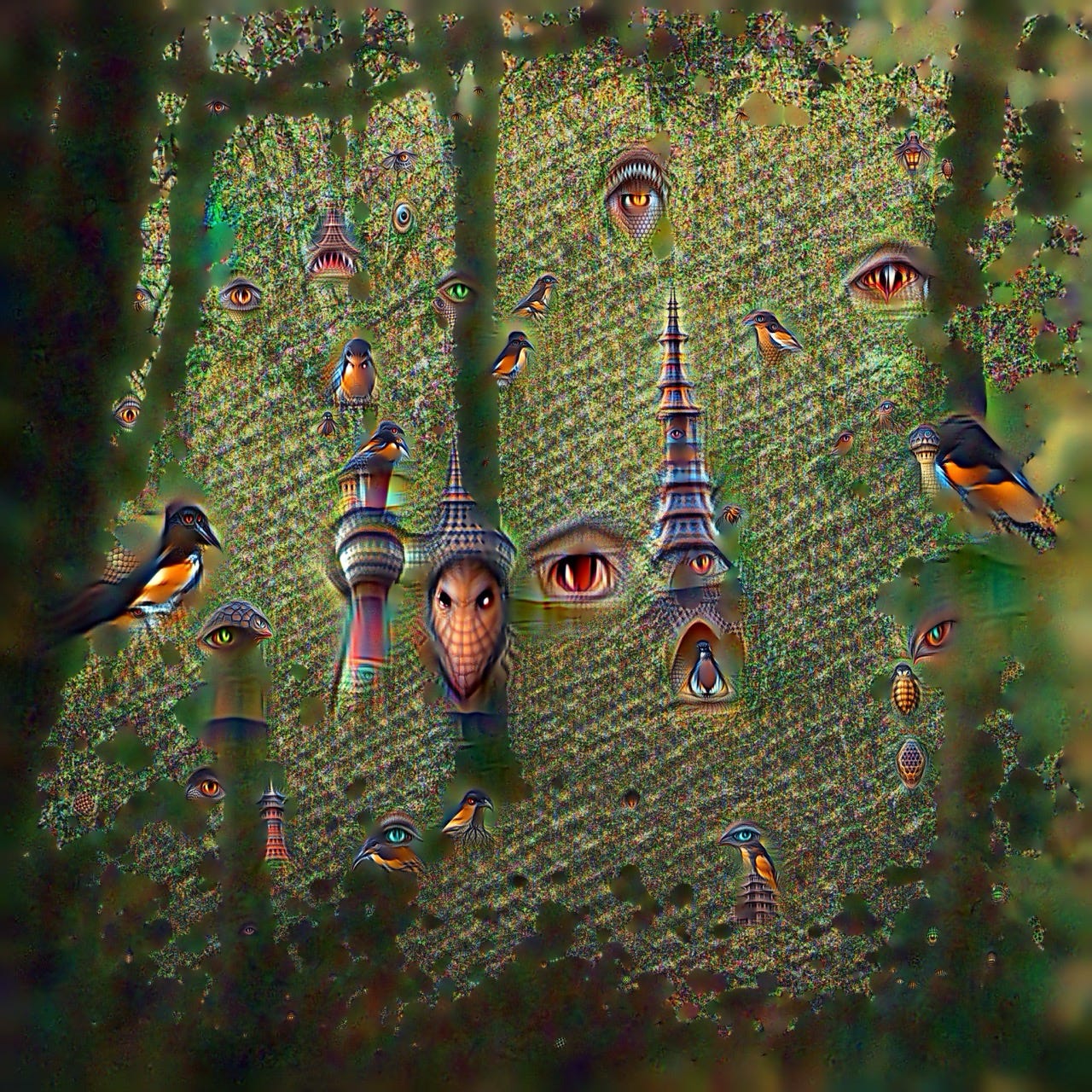
By using a Transformer backbone, the optimization process understands geometry. If we prompt for “Space,” a CNN might texture the leaves with stars. A Transformer is more likely to understand that the gap between the trees resembles a portal and place the nebula there. It optimizes for the concept, not just the texture.
5. The Viewport Problem: Cutouts and Robustness
If you show CLIP the entire image at once and optimize it, the model will cheat. It will find “Adversarial Examples”, tiny, imperceptible noise patterns that statistically look like the prompt to the AI, but look like static to a human.
To force the model to make human-perceptible changes, we employ a Multi-View Cutout Strategy.
Instead of processing the full image I, we generate a batch of N random crops (cutouts):
We resize these crops to 224x224 (CLIP’s native resolution) and optimize the average loss across all of them. This simulates looking at a painting from various distances and angles. If the model wants to minimize loss, it cannot just hide noise in the corner; it must ensure the target concept is visible in every random crop.
Augmentation for Stability:
To further prevent adversarial artifacts, we pass these cutouts through a differentiable augmentation pipeline before they hit the model:
Affine Transformations: Rotating and shearing the crops.
Perspective Warps: Tilting the view.
Noise Injection: Adding Gaussian noise.
This forces the optimization to find features that are invariant to transformation. A “heart” shape that disappears when you tilt your head isn’t a real heart. By punishing fragile solutions, we force the AI to paint robust, distinct features.
6. Topology-Aware Regularization
The most significant engineering challenge in Direct Optimization is High-Frequency Noise. The mathematical path of least resistance often involves creating jagged, “deep-fried” textures.
The standard solution is Total Variation (TV) Loss, which penalizes the difference between adjacent pixels, blurring the image.
The problem? Standard TV loss is global. It smooths the sky (good), but it also smooths the intricate bark of a tree (bad).
Our Solution: Weighted TV Loss
We implement a topology-aware masking system. Before optimization begins, we compute the gradient magnitude of the original image using Sobel Operators. This creates a map of “existing detail.”
We invert this map to create a Smoothness Constraint Mask (M):
High Value (White): Areas that were originally smooth (sky, walls).
Low Value (Black): Areas that were originally detailed (foliage, hair).
We then multiply our TV loss by this mask:
This creates a selective pressure. The optimizer is given free rein to hallucinate wild details in the textured areas of the forest, but is mathematically constrained to keep the sky smooth. This preserves the topology, the depth and form, of the original image while completely altering its texture.
7. The Octave Pipeline
Finally, we cannot optimize all frequencies at once. If we try to paint “hearts” on a 4K image immediately, the result will be surface-level noise.
We implement an Octave Schedule inspired by fractal mathematics.
Low Frequency (0.6x scale): We downsample the image. The optimizer shifts the global color palette and alters large shapes. The trees begin to bend.
Mid Frequency (1.0x scale): We upsample back to native resolution. The optimizer refines the edges of the new shapes.
High Frequency (1.4x scale): We oversample. The optimizer hallucinates fine grain details—the veins on a leaf become circuitry or stars.
More if needed…
At each step, we normalize the gradients. If the gradients are too steep, the colors explode (saturation clipping). We apply a tanh or soft clamp to the gradients to ensure the image evolves organically rather than violently.
Limitations
While this technique offers unique control, it comes with significant trade-offs that make it less practical than standard generation tools.
1. It is Slow: Unlike a Diffusion model which generates an image in a single deterministic pass (taking seconds), this is an iterative optimization loop. We have to run the model forward and backward hundreds of times for a single image. It is the computational equivalent of painting a portrait by hand rather than taking a Polaroid.
2. The “Deep-Fried” Danger: Neural networks naturally prefer high-contrast, high-frequency patterns. If we aren’t careful with our regularization (the smoothness masks), the optimizer will happily “burn” the image with neon noise and saturation spikes just to mathematically satisfy the prompt. This often results in images that look like corrupted JPEGs or “deep-fried” memes rather than art.
3. Dependency on Input: This is not a generator; it is a modifier. The algorithm is essentially lazy, it needs existing edges and shapes to latch onto. You cannot turn a plain white square into a complex landscape because there is no topology to distort. The quality of the hallucination is strictly bound by the complexity of the input reality.
Conclusion
When we ran the prompt “Love” on a forest image, the model didn’t just paste red clipart hearts on top of the leaves. Instead, it subtly twisted the existing branches and shifted the dappled sunlight until the forest itself looked like it was made of romance. It honored the reality of the original photo while completely changing the vibe.
This offers a surprisingly useful tool for AI research. By forcing the model to “draw” its thoughts onto an existing canvas, we get a direct look at how it visualizes abstract concepts, effectively letting us peek inside the black box.
We haven’t built a painter; we’ve built a pair of digital glasses. We can now look at any ordinary photo and force the computer to squint at it until it dreams a new meaning into the pixels.
Code:
https://github.com/Gal-Lahat/CLIP-DeepDream
hi Gal, please cek my DM.
very cool work!